Figure 1
Figures 1 and 2 are configured with the building giving total campus load; the secondary pump values are also shown for the total campus. The air handler and coil values are for one of the 45 units in the model. The plant values are also shown for one chiller/tower and pumps of the three-chiller/tower plant. The system performance and site kW demand data shown in the middle of the figure are for the total campus.
Figures 1 and 2 are configured with the building giving total campus load; the secondary pump values are also shown for the total campus. The air handler and coil values are for one of the 45 units in the model. The plant values are also shown for one chiller/tower and pumps of the three-chiller/tower plant. The system performance and site kW demand data shown in the middle of the figure are for the total campus.
Using ever-popular computer modeling, we look at the characteristics of a 1980s-era chilled water system. The exercise points out that you never really know how good the model is until the real thing is up and running, but it also entails a thorough look at the systems and their differences. The author also invites readers to “play along at home” and compare notes on their model results.
The purpose of a system model is to provide understanding of a system’s characteristics and performance under various conditions. A model that is to be used for system decisions should duplicate, within about 6%, measurements that can be made in the field on a real system, including temperatures, flows, cooling load, and kW demand of the components of the system.
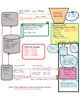
Figure 2
Designing a system defines most of the information needed for a system model. The model sets the design equations up as a set of simultaneous equations solved by computer. A system model on a laptop computer becomes a tool for checking the system after construction and during the life of the system. The model provides the tool to evaluate the system at commissioning and input the real system values into the model thereby providing control logic for the future operation and evaluation of the system.
The model presented here is not presented as the last version; model development is an ongoing process, with each real system providing new challenges and opportunities to better understand systems and models.
The System at Ideal Conditions
Figure 1 illustrates a 1980s system at ideal design conditions. The peak building load of 1,929 tons is less than the capacity of the plant, therefore, the three chillers are loaded to 98.5% of capacity, and the air handlers are operating at 36,490 cfm vs. the design of 40,000 cfm. The building is (830,000 sq ft), and the building cooling load of 1,929 tons comprises the values shown on Figure 1. The 45 air handlers are assumed to be equally loaded by the building load. The air distribution system is taken from option 1.1 At design, the air distribution unit is a 40,000-cfm VAV AHU with an overall design fan system pressure of 4 in. of water static pressure.Each VAV fan electric demand at design load is:
(fan)hp = (cfm) * dh/(6356 * Efan) = 40,000 cfm * 4.0 in./(6356 * 0.67) = 37.6 hp
(fan)kW = 0.746 kW/hp * 37.6 hp/ EASD-Mot. = 28.04 kW/0.82 = 34.2kW (at design load)
Where:
fan efficiency, Efan = .67
motor-VSD efficiency, EASD-Mot = .82
(Efan-ASD)= Efan * EASD-Mot = .67*.82 = .549 dh = fan static pressure (inches of water) = 4 in.
6356 = fan power constant

Table
1. Nomenclature.
Kavanaugh points out that the efficiency of the fan motor and adjustable speed drive (ASD) will vary with speed and torque. At 50% speed, the motor-ASD efficiency drops from the 82% indicated above to about 68%. The article also points out that the system does not follow the ideal system curve as (cfm) decreases. Figure 3 of Kavanaugh provides the reduction in fan pressure as the (cfm) decreases. These relations are in the model. The return air fan is assumed to be reduced by the ratio of the system (cfm) at energy equilibrium to the design 40,000 (cfm). The air handler (cfm) is calculated assuming the cooling load is all sensible loads.
Chapter 11, page 11.1 ofPrinciples of Heating Ventilation and Air Conditioning, states, “In most systems designed for human comfort, the system control responds to dry-bulb temperature, with the dehumidification being provided as a non-controlled by-product of the cooling process.”2
Option 1 of Kavanaugh also includes, for each of the 45 fans, powered terminals3 drawing about 24.1 kilowatts (kW). The fresh air fan is model as 0.72 kW for each of the 45 air handlers.
The coil is modeled as (UA) = 3.8 and capacity of (UA)*(LMTD), Delta T of 10°F, and 10 ft/sec water flow at design. The primary and secondary pumps are designed/selected for the values shown by the following equations.
(P)sec-kW= (7,200 gpm) * (348 ft.) * .746 kW/hp/(3960 * .80) = 590 kW
The model installed capacity of the secondary pumps is 700 kW.
(P)c-kW= (2,400 gpm) * (47.3 ft.) * .746 kW/hp/(3960 * .81) = 26.4 kW
The chiller is selected at 964 tons evaporator load, 85° water to condenser, and motor load of 566 for a 0.587 chiller kW/ton at design. The towers approach 7° at design wetbulb of 78° and 48 kW fan power.4
The shell load and fresh air load are modeled as approximately linear down to 60° where both loads are approximately zero. All electrical heat is modeled as loading the system 100% with the exception of the pumps. The pump electrical heat load is modeled as a function of the pump efficiency. The secondary pump heat load is 79.2% of 553.1 kW in Figure 1 and 72.3% of 233.6 kW in Figure 2. The chiller pump efficiency is 81%, and the tower pump is modeled as 83%.
Energy Equilibrium
Figure 1 gives the model values at energy equilibrium. The set of simultaneous equations has taken the building load of 1,929 tons and the design values and arrived at a steady-state condition. The result is that the air handlers and plant are not loaded to capacity. The obvious question: Is this a good model? The obvious answer: We do not know and will not know until the model is compared and evaluated against the real system in the field. If the model can be adjusted to agree with the real system then we have a good model; if not, then back to the drawing board, or rather, computer?Figure 1 is the ideal condition for the components and load as defined above. The controls on the system model are three. The air return temperature (Tar) is assumed as set at 76° for all 45 air handlers with an air duct pressure set at 3.8 in. water. The supply air temperature (Tas) is set at 58° and controlled by a valve on the return water from the coil. The secondary pump is assumed as controlled by a differential pressure (DP) sensor. Figure 1 is identified as ideal performance for several reasons, one being the unlikely possibility that the (DP) will control the secondary pump to give a load Delta T of exactly 10°.
Reduced Drybulb and Wetbulb Temperatures
Figure 1 gives the modeled response of the system at peak design load conditions that may never occur and certainly would not likely occur on the day the model is used in the commissioning or evaluation of the system.Three changes will be made to the model, the weather changed to drybulb 78°, and wetbulb 68°. These two weather changes result in the model shell load reducing to 491.2 tons and the fresh air load to 113.7 tons for a total building load of 1,305.4 tons, shown by Figure 2, vs. the 1,929 tons of Figure 1. The third change to the model is to adjust the chiller percentage to 59% or 333.9 kW to provide approximately 44° supply water.
A detailed comparison of Figures 1 and 2 illustrates that the performance of the system has been enhanced by the reduced load and lower wetbulb temperature. The chiller kW/ton has improved to .485 vs. .584 of Figure 1 and the site kW has decreased (7,441 – 6,109 = 1,332 kW). The reduced building load of (1,929 – 1,305 = 624 tons) first unloaded the air handlers resulting in a reduction of (2,783 – 2,441 = 342 kW). The reduced evaporator load of (2,863.5 – 2,066.1 = 797.4 tons) results in a plant kW reduction of (2,583 – 1,593 = 990 kW) for a total site kW reduction of (990 kW + 342 kW = 1,332 kW).
The change in drybulb and wetbulb temperature caused essentially all system values to change, arriving at a new state of equilibrium consistent with the laws of thermodynamics and the performance characteristics of the equipment and the defined building load. If the real system values, at these weather conditions, could be arrived at with the model by making adjustments consistent with the laws of thermo and equipment characteristics and measurements on the system, then we potentially have a good model. Model verification would require comparison at several conditions of the real system. A future article may deal with the analysis of a real system, beginning with the requirement that energy in equals energy out, minus change in internal energy of the system.
What If Analysis
Once a computer simulation of a system is developed, the ability to evaluate changes to the system is essentially unlimited. All energy consuming components of this 1980s-era system can be quickly and easily changed in the simulation to determine reduction in kW demand. Utilizing basic equipment of today, this system’s kW demand can be cut in half and the plant can be reduced to a two chiller/tower plant.The daily,weekly,monthly, season, or yearly energy use of the system can be estimated based on the kW demand of the system as the weather and building loads change. Weather changes are rather easy to estimate but turn down and turn off of lights and other loads are subject to people actions unless automatic turn off systems are installed. The point being that a computer simulation must be able to duplicate kW demand for given weather and building load conditions if it is to have a reasonable chance to estimate energy consumption over time.
Try It Yourself
If you are a system analyst, see what you get for the plant kW of Figure 2 if only two chiller/towers are operating; does plant kW increase or decrease and what is the chiller kW/ton and plant kW/ton? Try installing upgraded systems to Figure 1 and see how the site kW is decreased. Try evaluating the effect of low load Delta T, and then install P-only pumping. Try anything you like and e-mail me your analysis and I will give you my results. If you need more data, then make your own assumptions. Everyone is invited to “play” and who knows? We might learn something.ESReferences
1. Kavanaugh, S, “Fan demand and energy,” ASHRAE Journal, June 2000.2. Sauer, H.J. Ronald H. Howell, William J. Coad, “Principles of Heating Ventilation and Air Conditioning,” ASHRAE, Chapter 11 and Chapter 13, 2001.
3. The Trane Company, “Fan powered VariTrane,” Data Catalog, VAV-DS-9, pp.8, 50, 1995.
4. Marley Cooling Tower Company, UPDATE Version 4.12.1 and Version 4.12.2.