A colleague of mine was the project manager on a commissioning project for a build-out at a five-story, 150,000-sq-ft laboratory building at a large university. The commissioning team was finding it difficult to close out the commissioning process due to the poor performance of the exhaust air systems. The current construction project that they were commissioning consisted of the build-out of lab space on half of the fifth floor. The project had added about 40 fume hoods and now that construction was complete, the project could not be finalized because over one-third of the new hoods would go into a low-flow alarm condition when their sashes were raised beyond their minimum position.
The design engineering firm was under the belief that the central exhaust system, which was not modified during the construction project, was the cause of the issue. The project manager for the commissioning team realized that this issue could not be resolved until the root causes were understood. He requested that a coworker and I, who have experience in diagnosing complex building problems, visit the site and see if we could solve the problem.
Upon arrival, we met with the university project manager, the lead facilities engineer, and the TAB contractor. We soon learned that the building was only six years old and that the laboratory exhaust system had never performed well. It had performed just well enough in the past for the owner to occupy most of the building, but now that the fifth floor was completed, the exhaust system did not have the capacity to keep all of the 5th-floor laboratory hoods functioning properly. They also stated that even though the fans were located directly above on the roof, this floor had the poorest performing exhaust system, while the lower floors were performing adequately. This was counterintuitive because, typically, the systems furthest from the fan are ones to suffer the most.
We listened as the university project manager and the facilities manager conveyed their frustrations about the exhaust systems and hood alarms. Clearly, this was an issue that they had been fighting for quite a while. The TAB contractor then discussed his report and disclosed his theory about the exhaust system issues. He stated that the fume exhaust stack discharge cones were designed for an exit velocity of 10,000 ft/min, and the pressure loss from the cones was too high for the exhaust fans to overcome.
I had about 18 years of experience when we worked on this project. I knew that at 10,000 ft/min, the fans had to overcome a huge velocity pressure loss. The rule of thumb for fume exhaust stack discharge cones is around 3,000 ft/min, so you can imagine my curiosity when he stated that these stacks were designed for over three times the typical value. Armed with that information, we started our building tour.
When we arrived on the roof, we confirmed the exhaust design and duct sizes were consistent with the drawings and we recorded the nameplate information for the laboratory exhaust fans. Overall, there were a total of six laboratory exhaust fans. Each fan was sized for 60,000 cfm, making the total installed capacity 360,000 cfm.
Figure 1 shows the configuration that each of the exhaust fans, outside air intakes, dampers, and velocity cones were arranged in. While the fume exhaust system was variable volume, the fans were to be fixed at a constant speed while the outside air intake bypass damper modulated to maintain the exhaust manifold pressure at its pressure setpoint. Regardless of the fume exhaust demand from the building, the fume exhaust fans were designed to discharge 60,000 cfm at all times in order to maintain the stack velocity. It should be noted that the motorized outside air bypass damper was checked by both the balancer and controls contractor and found to be tightly closed.
We observed the velocity cones and noted that they appeared to be much smaller in diameter than the 60-in diameter exhaust ducts coming from the discharge of the fans. We could not get an actual measurement of the nozzles because they were too high in the air and the fumes being exhausted prohibited us from getting near them.
Back in the office, we started gathering data, plotting drawings, and crunching the numbers. We started by evaluating the capacity of the exhaust fans. When we were on site, we verified the fans to be direct-driven vane axial fans. According to the nameplate, each fan was designed to operate at 60,000 cfm against a total pressure of 4.8 in of water at a speed of 1,170 rpm, powered by 75 hp motors, and with blade pitch settings fixed at 23 degrees. We also confirmed that the fan performance characteristics were consistent with the original design drawings.
There is, however, one more step in this process. The capacity of this fan type is highly dependent upon the outlet configuration. Because of this, a correction factor must be applied to determine how much static pressure is available to flow the system. In this case, the outlet condition correction factor was calculated using the equation shown in Figure 2. The figure illustrates how the correction factor can be graphically determined and also lists the equation for determining the correction factor directly. In our case, the fans were installed with factory outlet cones so the “Ducted with cone” (line A) is what we used. We calculated the resulting correction factor of 0.43 in as shown below.
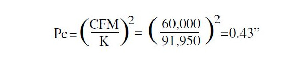
We calculated the final capacity of the fan pressure by subtracting the outlet correction factor from the fan total pressure as 4.80 - 0.43 = 4.37 in of water.
Next, we evaluated the velocity cones. Since we couldn’t directly measure the diameter of the outlet cones, we were lucky to get the sheet metal shop drawings from the original exhaust system infrastructure project. Using these, we were able to confirm that the outlet diameter of the velocity cones was 36 in. We then calculated that, if the fans were producing 60,000 cfm, the cone discharge velocity would be 8,488 ft/min.
I was then excited to calculate the pressure losses on the velocity cones and confirm how big of an impact they had on the system.
We looked up the loss coefficient from the ASHRAE Fundamentals Handbook. As shown in Figure 3, De = 36 in, D = 60 in, so De/D = 0.6, and therefore C0 = 8.10.
The design velocity of (V0) in the 60-in duct was 3,056 fpm, so we calculated the total pressure loss of the 36-in diameter velocity cones to be 4.72 in of water as shown below.

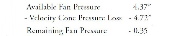
Recall that the fan at 60,000 cfm is only capable of producing 4.37 in of water pressure. If the velocity cone at 60,000 cfm has a pressure drop of 4.72 in of water, these fans with their velocity cones cannot produce 60,000 cfm. Simply put, the pressure loss from the exhaust stack alone was higher than the available fan pressure.
These velocity cones were, in fact, the guilty thieves. They were stealing fan pressure from the discharge of the fan, not allowing the pressure to be used on the suction side where it was needed.
Once we started reviewing the sheet metal shop drawings, another more subtle thief showed up. We quickly noticed that the branch ducts were connected to the main risers with sub-ducts penetrating into the riser. Figure 4 shows a riser diagram from the original drawings highlighting the sub-ducts. These were most likely added to satisfy a shaft penetration code condition, however, I’d never seen this applied to fume exhaust ductwork. Regardless, the issue is not with the existence of the sub-ducts, it is with how the sub-ducts were sized.
The fume exhaust riser as illustrated here was constructed as part of the original building and left in place for the future lab exhaust ductwork to connect in to. As each floor was finished, the fume exhaust ductwork was connected to the existing riser connection that was pre-sized by the original engineers. By the time the fifth floor was finished, the fume exhaust system was in operation and could not be shut down to change the size of the sub-duct. As a result, the design velocity of the sub-duct on the fifth floor ended up being 2,325 fpm. The sub-duct velocity for the remaining floors was much less than at this location so this fitting became a choke point in the system.
Similar to how we calculated the pressure drop for the velocity cones, we calculated the pressure loss for this sub-duct. Note that the inner corner of the square throat elbow is a sharp 90-degree turn. Figure 5 shows this corresponds to the radius being half of the width of the duct. The loss coefficient then becomes 1.06 because, in our instance, the duct happens to be four times thinner that it is wide (H/W = 4).
The design velocity at this location on the fifth floor was 2,325 fpm. The pressure loss from this configuration was P= C0 x PV,0 = 1.06 x 0.337=0.357 in of water. This is a high number for a single fitting but not an exorbitant value given the total of the system.
The other (less obvious) thief is the loss from the abrupt exit from the sub-duct into the riser. Figure 6 shows the loss coefficient for the abrupt exit as C0 = 1.0. The pressure loss from this configuration is then P= C0 x PV,0 = 1.0 x 0.337=0.337 in of water.
Note that the losses from the elbow and the abrupt exit taken together add up to 0.70 in of water pressure loss, which is 15% of the total anticipated system loss of 4.8 in of water.
This explains why the system could accommodate the exhaust needs of the lower floors but could not satisfy the floor closest to the fan. In this instance, just like the fume exhaust fan velocity cones, the thief is the velocity pressure.
In the design consulting business, it is sometimes too easy to estimate pressure losses based on rules of thumb, and with lower velocity systems, this strategy can be perfectly acceptable. One must be careful, though, because a conventional duct fitting may yield a pressure drop of a 0.1 in wc in one scenario and then rob a system of over 0.70 in of water pressure in a higher-velocity system. The difference is in the air velocity at the fitting. Speed kills. When the duct velocity is high, the stakes are high, and duct fitting pressure losses deserve a closer look. This project is a perfect example of where the effects of velocity pressure were overlooked with very expensive consequences.