My career in building energy management and energy modeling began in the fourth quarter of 1973 when the “Oil Embargo” occurred. I was a military systems design engineer with Texas Instruments Inc. (TI) and a member of a small group that simulated or modeled systems by computers for the purpose of design and evaluating the performance of the systems. The systems we modeled, for which I was personally involved with, included the Shrike missile flight and control, laser guided bombs, the gas dynamics of pneumatic actuators, cannon internal explosion and projectile exit speed, the dynamics and impact of electronics with soil, and the dynamics of metal compression. This experience led me to the task, in 1974, of modeling the energy consumption of TI buildings for the purpose of defining what could be done to reduce energy consumption. I used building energy computer programs available at the time that were based on simulating the yearly energy use of a building using utility bills. I became convinced that the need was for a building energy model that could model the last 24 hours of energy use and could also model the real-time energy use of a building at any hour. To accomplish this, a building energy model would require the same level of detail and sophistication as was required to model military systems. I spent years looking for this 24-hour building energy model, but it never appeared. Upon retiring, I decided to develop my own building energy model. Here is the first of a series of papers that verify the System Energy Equilibrium (SEE) Model.
(SEE) Model Objectives
The objective of the SEE Model is to duplicate the hourly performance of real systems at all operational conditions. To accomplish this, the SEE Model must obey the laws of thermodynamics and input the nonlinear characteristics of the real system components and model all details that contribute to the performance. The objective is to develop a math model, solved by computer, of the real system that duplicates the real-time performance at all operating conditions within about 3%.
Real-time models for control
System models are used for real-time control of systems as evidenced by NASA on space missions. Modeling the flight of a space vehicle after it has returned to Earth is too late. Similarly, modeling the energy consumption of a building over the past year is too late and impossible to perform with reasonable accuracy8. The need is for real-time, 24-hour building and plant energy models, and an SEE Model offers that capability.
Verifying the SEE Model Data
The development of the SEE Chiller Plant Model used three basic data sources to show the SEE Plant Model duplicates manufacturers’ data. First, Schwedler1 provides chiller/tower performance data for three plants as the load drops from a 1,000-ton design load down to a 300-ton load, and the wet bulb drops about 12°F below design wet bulb. Design wet bulb is different for each of the three cities. Second, the tower performance was verified against a manufacturer’s computer program for tower selection and performance3. Third, Trane2 provided chiller data that included the evaporator and condenser refrigerant approach temperatures, showing how it affects chiller kW. This Trane data was invaluable to the development of the SEE Plant Model.
Why Chiller Plant Model?
The first task of a chiller plant model is the design of the plant. The second task, after the plant is operational, is to answer the question, “Is the plant operating as designed?” This is a difficult question to answer because the plant may never operate at peak design conditions, and, if it did, would data be taken? An SEE Model of the plant offers the opportunity to visit the plant under any conditions of weather and load. The model will define performance compared to “as-designed performance” of the plant as it operates at part-load conditions. Third, if the plant is not operating as designed, then the SEE Model provides a tool to evaluate and define why plant performance is substandard. Fourth, the SEE Model provides a means of defining control strategies and may become part of the control software. Fifth, the SEE Model offers the ability to visit the plant in future years and define plant degradation due to aging, bad control practice, or other issues. Sixth, the SEE Model offers a design tool for defining, upgrading, or expanding the plant. And, seventh, a SEE Model provides the opportunity to evaluate issues raised by Engineered Systems and other HVAC publications. In summary a (SEE) Plant Model:
- Is a plant design tool.
- Answers the question, “Is the plant operating as designed?”
- Defines why plant performance is substandard.
- Defines plant control strategies.
- Defines causes of plant degradation.
- Defines upgrading or expanding of the plant.
- Models issues raised by technical publications.
This series of articles will show that the SEE Plant Model duplicates the chiller data of Schwedler, Trane, and Marley, verifying its performance. Model verification — the agreement of model with test data — was an absolute necessary step in my career as a designer of military products.
Building Plus Plant SEE Model
The principles of modeling demonstrated in this series of articles on plant modeling is applied to the modeling of a large office building defined by Pacific Northwest National Laboratory, Liu12. The building SEE Model10&11 has the ability to evaluate total building performance at real weather conditions13 and therefore provide building benchmark data at real weather conditions for any day. The fourth article in this series presents a brief discussion and a building plus plant schematic.
Chiller Plant Model Challenges
The challenge for the SEE Plant Model is to duplicate the data of Schwedler, Trane, and Marley. For a given city and design weather conditions, the tower is selected from manufacturers’ data3 and input to the SEE Model. The chiller is selected from manufacturers data2 and also input to the SEE Model. As load and wet bulb conditions change, the only input to the SEE Plant Model is a change in chiller kW required to provide the desired chilled water supply of, in this case, 44°.
The following figures present the data of Schwedler, Trane, and Marley, demonstrating the challenge for the SEE Plant Model; a challenge met as demonstrated by later articles in this series.
Figure 1 gives the evaporator load and wet bulb conditions for the three chiller plants1. The evaporator load is the same for all, but the design wet bulb and decreasing wet bulb values are very different, illustrating the challenge for the SEE Plant Model to duplicate tower and chiller performance within reasonable accuracy of 1%-3%. Schwedler defines the tower cold water approach to wet bulb as different for each plant. The Kansas City (KC) tower approach is 4°, Long Beach (LB) is 9°, and Salt Lake City (SLC) is 10°.
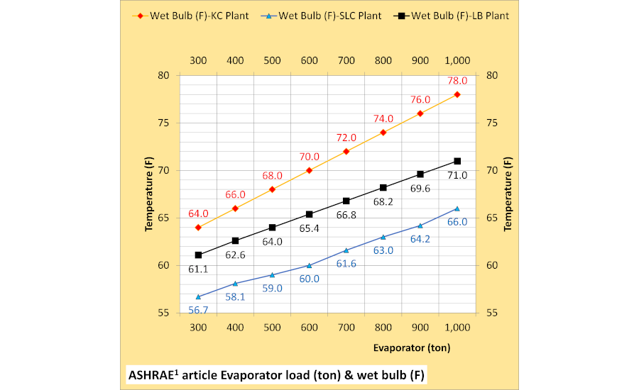
Figure 1. Evaporator load (ton) and wet bulb for three cities as defined by Schwedler.
Figure 2A gives the tower cold water or entering condenser water temperature (ECWT) at 100% tower fan speed, and Figure 2B for 50% tower fan speed. Figure 2A shows the ECWT for KC and LB is close to the same value with 100% tower fan speed, and Figure 2B shows the LB ECWT is greater than the KC ECWT when the tower operates at 50% fan speed.
These tower performance charts suggest the need for basic thermodynamic equations to model chiller/tower performance within 1%-3% given that the load on the tower is in part due to the chiller kW demand required to produce 44° supply water, i.e., the chiller/tower operate as one.
The SEE Model must go from Figure 2A to Figure 2B by changing only the tower fan speed and then adjusting chiller kW to get 44° supply water.
Figure 3A gives the chiller kW for 100% tower fan speed, and Figure 3B displays the tower at 50% fan speed. Figure 3A illustrates the KC plant demand is always greater than LB and SLC, and LB is always greater than SLC; however, positions change with 50% tower fan speed. Comparing the two charts illustrates the increase in chiller kW with 50% tower fan speed but also shows the chiller kW for LB is greater than KC down to 700-ton evaporator load. Figure 3 clearly illustrates a complex chiller/tower system requiring considerable detail in the thermodynamic equations to model Figure 3 performance within 3%.
Figure 4A gives the chiller kW/ton with 100% tower fan speed, and Figure 4B offers 50% tower fan speed. KC and LB change places at 1,000-ton evaporator load down to 700 ton with 50% tower fan speed. This shift in efficiency is due in part to chiller lift6. Chiller lift is the difference between the condenser refrigerant temperature and the evaporator refrigerant temperature6. Refrigerant temperatures are modeled by the SEE Plant Model as shown by the next article in this series.
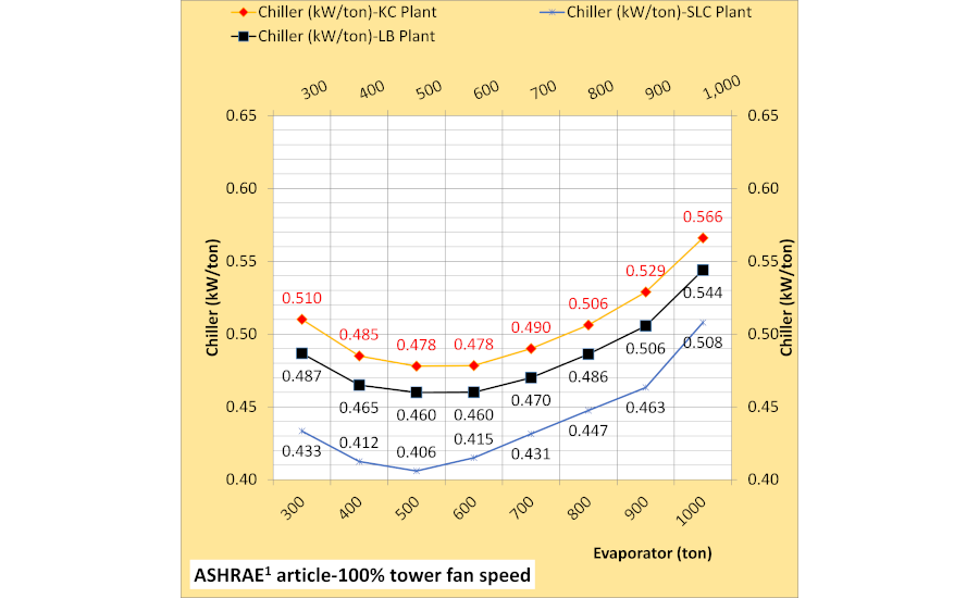
Figure 4A. Chiller kW/ton with 100% tower fan speed.
Figure 5 showcases the chiller plus tower fan kW per evaporator ton provided by Schwedler. Figure 5A, at 100% tower fan speed, illustrates the difference in kW/ton values for the three chillers/towers. Figure 5B, at 50% tower fan speed, illustrates the KC chiller/tower has about the same efficiency as the LB chiller/tower, and the SLC chiller/tower is the most efficient at both fan speeds. Figure 6 is the same data as Figure 5, but it gives the data per city, illustrating how the 50% tower fan speed changes the kW/ton of the chiller/tower. The KC chiller/tower with the 4° approach tower is more efficient with 50% tower fan speed at 1,000-ton evaporator load and below.
Both the SLC and LB chiller/tower become more efficient with 50% fan speed at about 800-ton and below evaporator load. The SEE Plant Model must duplicate this chiller and tower data of Figures 5 and 6 and does so within 3% as shown by future articles in this series.
Table 1 displays data at a 1,000-ton evaporator design load. Table 1 is data provided by Trane, showing the decrease in the evaporator and condenser refrigerant approach temperatures results in less chiller kW (column 19) required to produce 44° supply water of column 3. The reason chiller kW decreases and therefore chiller kW per evaporator ton decreases (column 20) is the drop in chiller lift as the refrigerant approach temperatures of the condenser and evaporator decrease. Chiller lift (column 18) is defined6 as the difference in the condenser refrigerant temperature (column 17) minus the evaporator refrigerant temperature (column 9). Chiller lift is addressed in detail in Part 2 of this series. The columns shown in yellow are inputs to the SEE Plant Model, and the other values must be duplicated by the model.
The next three articles in this four-part series show that the SEE Plant Model duplicates the Schwedler, Marley, and Trane data within 3% and most data within 1%-2%. The purpose is to establish the validity of the SEE Plant Model so design and performance decisions can be made and design and control strategies can be installed in a given plant.
What’s Next?
Part 1 of this series has defined the challenges for the SEE Plant Model and duplicates the Schwedler, Trane, and Marley data. The evaporator load decreases from 1,000 ton down to 300 ton as the wet bulb decreases about 12° for both 100% tower fan speed and 50% tower fan speed. Computer simulating the Schwedler data required a very detailed set of chiller/tower equations that will be demonstrated by Parts 2, 3, and 4.
Table 1 is equally demanding of the SEE Model, requiring a detail model of the chiller condenser and evaporator refrigerant temperatures so that chiller lift can be defined. Part 3 will address this challenge.
Part 2 will show that the SEE Model duplicates the Schwedler Kansas City data that requires a detail chiller model coupled with a detail tower model. The chiller performance is dependent on the tower, and the tower performance is dependent on the chiller. These papers generally refer to chiller/tower performance.
An example of applying the SEE Plant Model can be reviewed by clicking http://kirbynelsonpe.com and click on “Prescription for Chiller Plants7.” Perhaps the greatest value of a 24-hour SEE Model is the ability to energy benchmark a building against real weather13 data on any day. Energy benchmark analysis of several cities can also be reviewed at the above site11.
References
1. Schwedler, Mick. July 1998 “Take It to The Limit…Or Just Halfway?” ASHRAE Journal.
2. Trane chiller selection data received by Kirby Nelson from Springfield Missouri Trane office.
3. SPX Cooling Technologies (Marley). UPDATE Version.
4. “Introduction to Thermodynamics and Heat Transfer.” 1956 Prentice-Hall, Inc. by David A. Mooney.
5. “Thermal Environmental Engineering,” third edition. 1998 Prentice-Hall Inc. by Thomas H. Kuehn, Chapter 3.
6. 2012 ASHRAE Handbook, “HVAC Systems and Equipment,” Page 43.10, Figure 11, Temperature Relations in a Typical Centrifugal Liquid Chiller.
7. Mark Baker, Dan Roe, Mick Schwedler. ASHRAE Journal June 2006. “Prescription for Chiller Plants.”
8. ASHRAE Journal May 2016. “Modeled Performance Isn’t Actual Performance.”
9. Nelson, K. “Simulation Modeling of a Central Chiller Plant” CH-12-002. ASHRAE 2012 Chicago Winter Transactions.
10. Nelson, Kirby. July 2010 “Central-Chiller-Plant Modeling” HPAC Engineering.
11. Nelson, Kirby. “System Energy Equilibrium (SEE) Building Energy Model Development & Verification,” http://kirbynelsonpe.com.
12. Liu, B. May 2011. “Achieving the 30% Goal.” https://www.energycodes.gov/sites/default/files/documents/BECP_Energy_Cost_Savings_STD2010_May2011_v00.pdf.
13. Real weather data www.wunderground.com.
14. Taylor, S. 2011. “Optimizing design & control of chiller plants.” ASHRAE Journal (12).