Control charts have been widely used for monitoring production processes and identifying assignable causes of variability. Many papers investigate the application of control charts in different business situations, such as: improving inventory accuracy (Hart 1998); monitoring the diesel consumption for trucks (Akcakoca and Sutcu 2010); monitoring paper production (McSweeney 2006); monitoring plasma processing equipment (Baik et al. 2009); tracking physicians productivity (Lighter and Tylkowski 2004); predicting workplace health outcomes (Nunes et al. 2011); monitoring financial reporting of public companies (Dull and Tegarden 2004); analyzing data from student evaluations of teaching (Marks and O'Connell 2003); and analyzing crime rates in Houston(Anderson and Diaz 1996). In this paper, we present an example of how control charts have been used to monitor the room temperatures and to improve the operations of the BAS at Slippery Rock University.
Problem
In 2009, a new BAS for monitoring and controlling the room temperatures was installed at Slippery Rock University. The system takes readings of the temperature in multiple spaces (classroom, office, auditorium, closet, storage area, etc.) in buildings across campus. When the outside temperature rises above a set temperature (between 50° to 60°, depending on the building HVAC system), the air conditioning mode is activated. When the outside temperature drops below 50°, the heating mode is activated. When the outside temperature is between 50° and 60°, the system may be in “neutral” mode, depending on the heating/cooling building setpoint.
Even though the system allows predetermined setpoints, the actual temperature in the space was much lower or much higher than the room setpoints. The university was incurring high heating/cooling costs due to lack of control in the building HVAC systems or room thermostats. A project was launched with the goal to determine whether the space temperature was in control and to identify ways to avoid unnecessary heating or air conditioning costs.
Data collection
The project started with a visual inspection of all spaces controlled by the BAS, taking pictures of the factors affecting the temperature, and asking people using the space about their satisfaction with the room temperature. The BAS contained historical data on the daily temperature readings, taken every 15 minutes for 12 months (8 months for some spaces). The BAS also contained the individual spaces current setpoints. These setpoints were the temperature targets used as specification limits in the analysis. For example, if a room setpoint was 72°F, then the specification limits were computed as the setpoint +/- 2°, resulting in a lower specification limit (LSL) of 70°F and upper specification limit (USL) of 74°F.
Data analysis
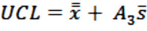
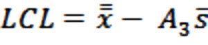
Usually, -chart and R-charts are used for continuous variables, however, when the number of observations (n) is greater than 10, it is recommended to use an -chart instead of R-chart. -chart and s-chart were constructed by computing the center line (CL), upper control limit (UCL), and lower control limit (LCL) for each month. For example, June has 30 days, corresponding to 30 samples. Each sample (each day) contained 40 observations (10 occupied hours * 4 readings/hour), resulting in a sample size of 40. The following formulas construct the control limits:
- The x-chart control limits:

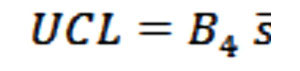
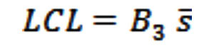
- The s-chart control limits:

where A3, B3, and B4 are constants, computed with the following formulas:
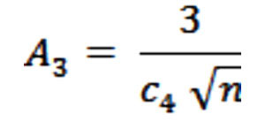

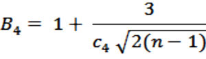
where,
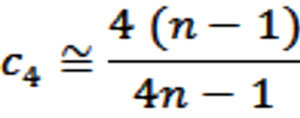
For example, the -chart control limits for the choral room in June are: UCL = 70.77, CL = 70.24, LCL = 69.77. The -chart control limits are: UCL = 1.48, CL = 1.10, LCL = 0.72. These limits were computed with constants: C4 = 0.98, A3 = 0.48, B3 = 0.65, b4 = 1.34. Figures 1 and 2 represent the s-chart and the -chart; both in-control.
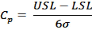
The next step computes the process capability indexes, which reveal if the process is capable to meet the specifications. For the choral room the setpoint is 70° with 2 degrees tolerance. Thus, the LSL = 68 and USL = 72. The following formulas compute the process capability indexes:
Process Capability Ratio:
Process Capability Index:
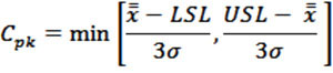
Cpk represents the distance of the process center to the nearest specification limit in units of the process width. Cpk is positive when the process mean is inside the specifications; Cpk drops to zero as the mean hits the USL or LSL. For our example, Cp = 0.61 and Cpk = 0.53; the process mean is almost at the specification center. However, as Cp = 0.61, the process is not capable; some days the temperature drops below the LSL or rises above the USL. Figure 3 illustrates this case.
Using the same method, we construct the control charts for all months for all spaces and compute the process capability indexes.
Results
Analysis reveals several situations:
-
Process in-control and capable (~2% of the cases). No need for change.
-
Process in-control but not capable (~13%). Look at choral room (Figures 1, 2, and 3). Two options exist: (i) reduce the process standard deviation and (ii) revise the specification limits. In the choral room case, revision of the limits is a preferable solution, as this will not affect the customer satisfaction. The choral room is spacious, used by many people, and if the tolerance is increased from 2° to 3°, the process will be almost capable (Cp = 0.91, Cpk = 0.84) and with higher customer satisfaction.
-
Process out of control due to identifiable special cause (~49%). The process is out-of-control due to three main causes: (i) turning the HVAC system off during the weekends, (ii) turning it off during the holidays, and (iii) high variability in external temperature. Figures 4 and 5 illustrate the situation when the temperatures go above the upper control limit every seventh day. In July, the facility turns the air-conditioning units off for the weekend, as the classroom is not in use. The weekend readings during unoccupied times should be removed from the analysis and new control limits calculated.
-
Figures 6 and 7 illustrate similar situations with average temperatures on the first, second , and third of January, way below the lower control limit. During these three days, the university was closed for the winter break and the heating was turned off. These three-day readings should be removed from the analysis and new control limits calculated.
-
Figures 8 and 9 present a situation where the temperatures are out of control due to rapid changes in the outside temperature, usually during the spring and fall months. One may argue that the outside temperature is not a special cause, as the goal of the heating/air-conditioning is to keep the inside temperature constant despite the outside temperature amplitudes. Internal and external temperatures, however, are highly correlated. That is why the external temperature during the months with high amplitudes is a special cause. Adjusting the process during these months is difficult, as the heating/air-conditioning units are set up to respond to the changes in the external temperature. The situation is even more complicated when the system transitions back and forth between heating and cooling modes.
-
Process out of control due to unidentifiable special cause (~36%). Figures 8 and 9 illustrate that the auditorium’s November out of control temperatures are not related to the outside temperatures. Management needs to investigate and correct the problem on that specific date. Common problems include power outages (requiring restarting the variable frequency drives controlling the fan motors of the air-handling unit) or failure of the building air compressor (provides control air).
Table 1 summarizes the results for all spaces for each month. In approximately 85% of the cases, the temperature was out-of-control, except for the choral room, where the temperature was in-control most of the months. Band room, classroom, and library reading room temperatures were, in general, higher than the setpoints. Alumni house meeting room 1 temperatures were lower than the setpoint. Auditorium, alumni house offices, alumni house meeting room 2, and cafeteria temperatures were outside the specification limits.
The winter break, with the HVAC systems turned off, forced the January room temperatures out of control. High outside temperature fluctuations forced April and May room temperatures out of control. The cooling/heating modes come from the same system, but are activated depending on the outside temperature. High outside temperature fluctuations result in high inside temperature fluctuations as the system goes back and forth from cooling to heating mode. Similarly, in June, high outside temperature fluctuations and the HVAC system off during the weekends lead the process out-of-control (above the upper control limit). In July, the air conditioning is turned off during the weekends, resulting in out-of-control temperatures (above and below the control limits). In August, low occupancy and the HVAC system turned off at different times, forced temperatures out-of-control. In September, when the classes resume, the temperatures go out-of-control due to the system adjusting to the weather changes. In October, the temperatures are out-of-control and much lower than the setpoint. In November, the temperatures are out-of-control and much higher than the setpoint. In December, the temperature is again out-of-control, due to turning off the heating during the weekends.
Recommendations
Based on the analysis, the following conclusions and recommendations are made:
-
Process standardization. The setpoint for the meeting room 1 was 74° and for meeting room 2 was 70°. The more consistent the setpoints, the easier the process control.
-
Tolerances. Many of the control charts were out-of-control, much higher or lower than the specification limits because of the narrow specifications limits. When the specification limits are set with one-degree tolerance (auditorium and classroom), increase the tolerance from one to two degrees. Small increase in the tolerance, irrelevant to the customer, will make the process capable.
-
Process mean higher than the specification target. When the process mean is higher than the specification target, reset the setpoint. For example, in the library reading room, the temperature was consistently much higher than the setpoint of 72°. It is a closed space, with no windows, with computers and a printer constantly in use, generating a lot of heat, which makes the space hot and uncomfortable to use. Reducing the setpoint to 70° or 68° will partially solve the problem, as the heat around the space during the heating season is enough.
-
Process mean lower than the specification target. Similarly, for those spaces where the process mean is lower than the specification target, the setpoint could be reset based upon occupancy. Meeting room 1 had temperatures much lower than the specification limit, especially during the summer months. The setpoint was 74°, but the room was kept much colder with the airconditioning running at full power, even when the space was not in use. Similarly, the classroom was not in use during May, June, July, and August, but had a cooling setpoint of 70°. In this particular case, the university is wasting money cooling a space that is not in use. Either reset the setpoint to a higher temperature, based upon room occupancy, or turn the unit off when the space is not in use. Shade the windows to block the sun during the summer months.
-
Redesigning spaces. The cafeteria is a large space with an automatic door at the main entrance. The door is constantly open as people go in and out. In this case, the outside temperature influences the inside temperature, making the place cooler in winter months (December) and warmer in summer/fall months (June, July, August, September, and November). Currently, the employees are using individual electric heaters to stay warm during winter months, causing more fluctuations in the inside temperature and incurring additional costs for the university. One possible solution is installing an air curtain serving as a shield against the cold blast coming in through the doors. Another solution, although more expensive, is redesigning the exterior entrance so the west winds are not entering the lobby when people enter the building. Placing window shades will also reduce the sun impact and improve the temperature control during the summer months when the space tends to overheat. Similarly, meeting room 2 was directly exposed to outside airflow through the entrance doors, resulting in the process being out-of-control all the time. Adding a second set of doors could improve the temperature control in this space.
-
Allowing users to adjust the temperature. In several spaces, the thermostats were either broken (classroom) or deliberately removed (meeting room 1) to limit the users control over the temperature. The idea was to prevent people from adjusting the setting and to interfere with the room temperature control. Allowing the classroom users to reduce the temperature in November, however, would have saved the university money on heating.
-
Consider the thermostat location. The thermostat location tremendously affects the readings. For example, the library reading room thermostat is located directly under the air vent. The alumni house office’s thermostat is located high in the center of a wall picking up the warmer air in the room, resulting in readings that are higher than the temperature that people actually feel in the room. When not practical to change the thermostat location, consider it when determining the room setpoints.
Finally, to illustrate better the causes of the out-of-control temperatures, a cause-and-effect (Fishbone) diagram is presented on Figure 12. The causes are classified in different categories: people, measures, methods, environment, thermostat, and space design. It may not be possible to control the outside temperature (environment) or to change the space design, but the rest of the categories provide opportunities to improve room temperature control.
Conclusion
This study presents the application of control charts to monitor the room temperatures at Slippery Rock University and provides important results and recommendations to the facility management. The fact that most of the control charts were out of control points to the need to reevaluate the factors affecting room temperatures to standardize the process and to determine setpoints and tolerances of the system. Given the complex nature of the task and the numerous factors interrelated in the room temperature, it is advisable to start with a basic evaluation of the most common spaces and to reevaluate them annually to reflect any changes in the usage and the space design impacting the temperatures. As this was the first time the facility analyzed temperature readings, the study became a pilot one for further analysis. Results showed that monitoring room temperatures provides useful insight into the process and identifies several ways to improve customer satisfaction and save money at the same time. We believe that the methodology of the analysis and the results could be used by other facilities at different institutions.
References
Akcakoca, H., and N. Sutcu. 2010. Investigation of the diesel consumption for trucks at an overburden stripping area by SPC study. Journal of Applied Statistics, 37 (2): 283-298.
Anderson, E. A., and J. Diaz. 1996. Using process control chart techniques to analyze crime rates in Houston, Texas. Journal of the Operational Research Society, 47 (7): 871-881.
Baik, S., W. Kim, and B. Kim. 2009. In-situ detection of plasma processing equipment using a V-mask control chart. Materials & Manufacturing Processes, 24 (12): 1418-1422.
Dull, R. B., and D. P. Tegarden. 2004. Using control charts to monitor financial reporting of public companies. International Journal of Accounting Information Systems, 5 (2): 109-127.
Hart, M.K. 1998. Improving inventory accuracy using control charts. Production and Inventory Management Journal, Third Quarter: 44-49.
Lighter, D. E., and C. Tylkowski. 2004. Case study: Using control charts to track physician productivity. Physician Executive, 30 (5): 53-57.
Marks, N. B., and R. T. O'Connell. 2003. Using statistical control charts to analyze data from student evaluations of teaching. Decision Sciences Journal of Innovative Education, 1 (2): 259-272.
McSweeney, L. A. 2006. Monitoring paper production using a spectral control chart designed to detect in the presence of multiple cycles. Journal of Applied Statistics, 33 (5): 467-480.
Nunes, I. L., J. J. Larsson, B. J. Landstad, H. H. Wiklund, and S. S. Vinberg. 2011. Control charts as an early-warning system for workplace health outcomes. Work, 39 (4): 409-425.
Acknowledgements
We would like to thank all students from Total Quality Management class of spring 2011 at the School of Business at Slippery Rock University for their help with cleaning, tabulating, and analyzing the data for this paper.