Calculating the Power Consumption of Heat Recovery Chillers with a Variable Temperature Campus Water Loop

Chillers have typically been thought of as providing cold water to cooling coils located in a variety of air-handling systems throughout a building. However, there are certain building owners and operators who put a high value on energy reduction and sustainability. Heat recovery chillers (HRC) and water-to-water heat pumps are one way to improve the energy efficiency of a building’s mechanical system, as these systems reuse the energy in the system before the energy is rejected to the atmosphere.

It’s important to find an accurate method to calculate the power consumption of an HRC to better validate system efficiency. Most energy modeling software on the market does not support the simulation of an HRC system, especially when the chilled water source is supplied from a variable temperature campus loop. This is the challenge the authors faced during a recent project, as they worked to develop a way to accurately model these systems. This article explains how to accurately model an HRC system that is connected to a variable temperature campus water loop.

HVAC System Description

HRC central plants can be piped in a variety of ways depending on what the driving factors are for a heat recovery system, including building type, use, load, and the climate a structure is located in. A traditional piping arrangement to supplement a domestic hot water system or HVAC heating hot water system is shown in Figure 1. The chilled water system is piped in a traditional manner. The condenser water system is piped to the domestic hot water system or the HVAC heating hot water system. It’s important to note that a heat exchanger is required for domestic hot water systems. A double-wall heat exchanger should be used to ensure the water systems do not mix and cause a health issue in the domestic hot water system.

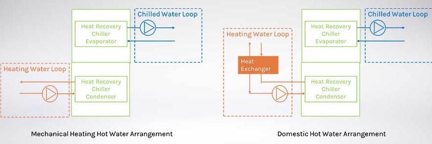
FIGURE 1. A typical heating heat recovery chiller arrangement. Images/tables courtesy of SmithGroup

The central plant piping arrangement for the case study substitutes a heat exchanger in place of a traditional condenser water system. Heat exchangers decouple the building from the campus central plant. Multiple HRCs are provided in a parallel arrangement that would allow individual HRCs to operate in cooling or heating mode. A water transfer loop between the heat exchangers and the HRCs enables the independent operation of the HRCs. Figure 2 indicates the piping diagram for this system.

FIGURE 2. An HRC system with a campus water loop.

Methodology

The most important parameter is the hourly coefficient of performance (COP) when calculating the HRC energy usage. The HRC heating and cooling energy usage can be calculated by using the hourly building heating and cooling load:

Chiller heating power = heating load / heating COP
Chiller cooling power = cooling load / cooling COP

In addition to the aforementioned energy usage, the hourly heating or cooling load rejected to the campus water loop needs to be provided to the campus engineers. This is so the effect of a new building load connecting to the campus central systems can be assessed by the campus staff to meter and monitor the building load and assess the campus central plant operations.

3.1 Coefficient of Performance

What is COP, theoretical COP, actual COP, and relative COP? The COP of a chiller is defined as the ratio of the total heating or cooling provided to a system compared to the work done by the refrigeration system. The theoretical COP is related to the condenser water temperature and evaporator water temperature of the chiller. The relationship between COP and condenser and evaporator temperature is shown in the formulas below:

COP _heating = T _condenser / (T _condenser – T _evaporator)
COP _cooling = T _evaporator / (T _condenser – T _evaporator)

The mechanical process is not 100% efficient, and there is always heat loss during the actual operation process. The actual COP is always slightly lower than its theoretical COP, which is also known as Carnot COP, from the Carnot refrigeration cycle. It is a function of the upper and lower temperatures of the cycle, which is equal to the condenser and evaporator temperature. The reverse Carnot cycle is the most efficient refrigeration cycle operating between these two specified temperature levels. A coefficient η is utilized as the ratio of actual COP to the theoretical COP. This is known as the relative COP.

3.2 Relative COP to Part-Load Ratio Curve

Relative COP, η, is related to the part-load ratio for a given HRC. The relative COP at different part-load ratios needs to be calculated based on the data provided by the chiller manufacturer to obtain the relative COP curve.

Table 1 is an example of the given manufacturer HRC performance curve.

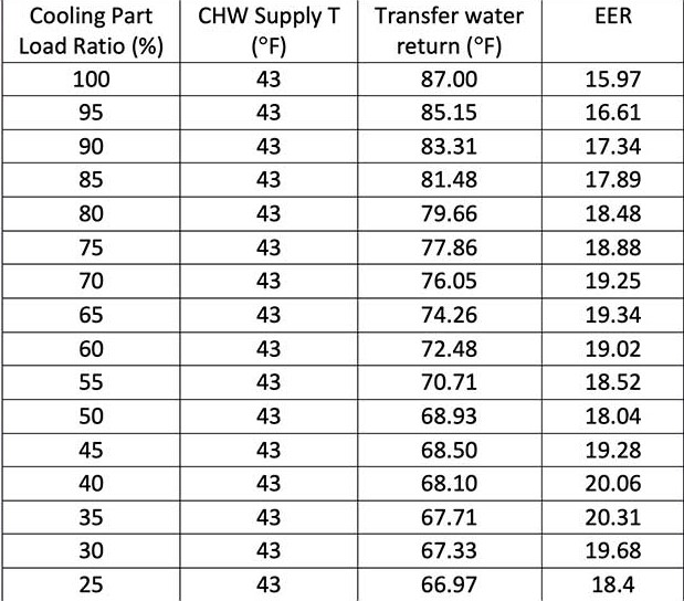
TABLE 1. Manufacturer heat recovery chiller part-load data.

The relative COP at different part-load ratios needs to be calculated based on the actual COP and EER at different cooling part-load ratio.

η = COP _{cooling, theoretical} / COP _{cooling, actual}COP _{cooling, actual} = EER / (3.412)

The theoretical COP at different cooling part-load ratios can be calculated based on the condenser and evaporator temperature.

COP _{cooling, theoretical} = T _{evaporator, manufacturer} / (T _{condenser, manufacturer} – T _{evaporator, manufacturer})

The condenser and evaporator temperature can be calculated based on the given chilled water supply temperature, transfer water return temperature, and approach temperature.

T _{evaporator, manufacturer} = T _{CHW supply, manufacturer} – T _{approach, manufacturer}
T _{condenser, manufacturer} = T _{transfer water return, manufacturer} – T _{approach, manufacturer}

3.3 Theoretical COP with Campus System Water Temperature

Temperature differences between the various systems need to be accounted for in both the heating and cooling applications. This case study has various water systems that heat is transferred through with the decoupling heat exchangers and the transfer water loop. The system was designed with a 2°F approach for the heat exchangers that decouple the building from the central plant. Similarly, approach temperatures in the transfer water loop and in the HRC need to be accounted for between the evaporator and condenser. The system was designed for 8° and 4°, respectively. Approach temperatures and system delta Ts will vary based on conditions for specific applications.

Result Analysis

4.1 Relative COP (η) to Part-Load Ratio Curve - Using the aforementioned methods, the relative COP was able to be calculated from the HRC manufacturer’s part-load curve. In Table 2, the HRC manufacturer’s data is shown in the green columns, and the white columns indicate the system water temperatures after heat is transferred between systems and the resultant COPs. The relative COP is the highest at and near full-load operation, and there is a significant drop off at approximately 60% part-load operation of the HRC.

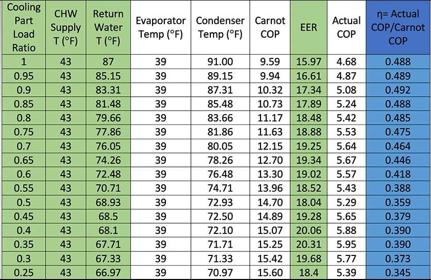
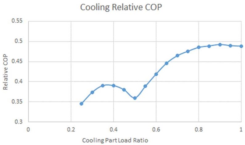
TABLE 2. The process of calculating relative COP in cooling operation.

FIGURE 3. Relative COP in cooling operation.

Figure 3 displays the relative COP curve, η, which shows the effect of lowering the cooling part-load ratio from the manufacturer’s part-load curve.

Similarly, Figure 4 is the relative COP curve, η, which shows the effect of the heating part-load ratio from the manufacturer’s part-load curve.

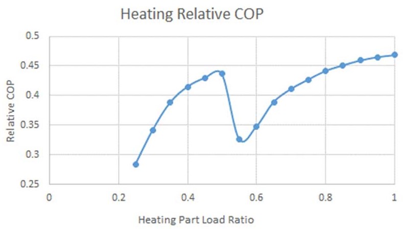
FIGURE 4. Relative COP in heating operation.

With the curves shown in Figures 3 and 4, the relative COP, η, valve can be understood with cooling or heating part-load ratio in actual operation mode.

4.2 Hourly Building Heating and Cooling Load

The annual building load must be calculated to determine the mechanical equipment sizes and determine the energy efficiency of the proposed building envelope, mechanical system, and lighting system. This can be calculated using any building performance simulation software. Figure 5 shows the annual building load for the project referenced in this article.

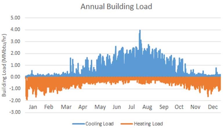
FIGURE 5. Annual heating and cooling load.

The part-load ratio is equal to the cooling load or heating load divided by the peak cooling or heating load. This assumes all HRCs are operating at same part-load ratio. The hourly relative COP valve can be read from that and the curve referenced under section 4.1

4.3 Hourly Chiller Heating and Cooling Energy

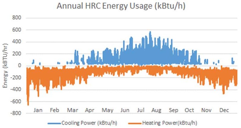
For this case study, Figure 6 shows the annual cooling and heating HRC energy consumption, which is 389 MBtu per year in cooling mode and 549 MBtu per year in heating mode. This shows the benefits of redistributing the heat in the system prior to rejecting the heat to the atmosphere or, in this case study, back to the campus central plant. This also makes full use of the mild temperature campus water. The mild temperature campus water makes it possible to recover heat from the central plant side, which increases the campus overall efficiency.

FIGURE 6. Hourly heating and cooling HRC power.

4.4 Hourly Heating and Cooling Load to the Campus Water Loop

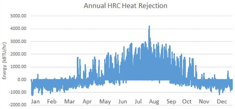
By using the aforementioned methods, the amount of heat rejection from the building to the campus chilled water system can be calculated. The hourly heating and cooling load returned to the campus chilled water loop is the difference of the heat rejection by the HRC and the adsorption by chiller. Figure 7 shows the net heat rejection to the campus central plant (shown as a positive) and the net heat absorption from the central plant (shown as a negative) from the campus water loop, in which the total heat rejection is 2,443 MBtu per year, and the total heat adsorption is 951 MBtu per year.

FIGURE 7. Building load to the campus central plant.

Conclusion

HRCs and water-to-water heat pumps can provide significant energy savings over traditional central plant arrangements. This is important as the HVAC industry continues to serve as a leader in sustainability and overall energy reduction goals. Being able to accurately model these systems will lead to better system operation. This will be done by being able to predict cooling and heating coincident loads as well as when and how much of the loads will need supplemental cooling or heating. This will allow engineers to properly size equipment to maximize the efficiency of the overall mechanical system.