
In 2010, looking for a way to improve plant performance, HGA sat down to write an equation to describe the total energy use of a chiller plant. The plant at hand consisted of three different chillers, only one of which used a variable-speed drive. Thirty pages later, HGA had a clearer understanding of the degrees of freedom available to impact energy use, the interactions between components, and a realization that the performance ultimately came down to how engineers respond to two independent parameters: 1) system load; and 2) Outdoor air wet bulb temperature (Toawb). For any given load and Toawb, there is a most efficient set of operating parameters that result in the lowest energy use for the entire the plant. This is the Best Efficiency Point (BEP).
Predictive Optimization
If engineers can determine the BEP for every possible operating load and Toawb and reduce this to a series of set point equations, they have a repeatable optimized operating strategy.
The purpose of a central cooling plant is to aggregate and serve loads in an efficient manner. If engineers maximize the efficiency of the plant at the cost of space comfort for the users or process performance, they have not done their job well. It is almost always more efficient to operate at a higher chilled water supply temperature (Tchws). Tradeoffs of pumping energy and chiller energy can be determined in the plant, but the impact on space humidity and temperature must be considered. The magnitude of total fan energy is generally about equal to chiller plant energy, so reducing plant energy is not a net gain if the fan energy increase offsets plant savings. The optimization falls short if the spaces served are no longer within design parameters.
Operating limits became a concern when the industry made the shift from primary-secondary pumping to variable-primary plants and later applied flow variations to the condenser water system. To gain the greatest efficiency from a plant, all parameters should be variable, but all parameters have limits. Typically, the limits of concern are minimum and maximum flows, but equipment turndown as a function of operating conditions also comes into play. This is sometimes a challenging part of programming a variable-speed plant, because respecting the limits is important. On the low end, a minimum flow protects equipment, prevents freezing of tubes or fouling of cooling towers, limits heat transfer degradation, and keeps pumps in a controllable range. On the high end, a maximum flow avoids excessive pressure drops, loss of temperature control, overflowing towers, and tube erosion.
Chiller degradation takes place both seasonally and over time. Tubes foul, air is introduced into low-pressure machines, or refrigerant is lost in high- or low-pressure chillers. Each of these tends to increase the evaporator and condenser approach. A higher approach means the chiller operates under greater lift, but the BEP, at the inflection point of the curve, moves very little since the curve is a function of the compressor. As mechanical seals wear, refrigerant leakage may be affected, but the curve inflection maintains its position defined by other parameters. If chiller efficiency drops, the chiller uses a larger fraction of the total plant energy — just as if strainers start to foul, pumping energy increases, and pumping energy has a slightly higher proportion of total plant energy. In each case, the relative energy use of chillers versus auxiliaries has generally the same characteristics and plant BEPs. The point here is not to ignore plant degradation but to demonstrate that predictive optimization remains valid even as a plant degrades. Plant maintenance and tracking are important to maintain peak efficiency.
So, by measuring two parameters, Toawb and load, engineers can establish the repeatable BEP of the plant without the complexity of the active controls or a machine learning approach. This makes high-efficiency plants available to direct digital control (DDC) systems at a much lower cost without third-party control boxes. It’s the same technology distilled to a set of operating curves programmed into the control system.
Responding to Opportunities On-Site
The first predictive optimization principle, that the plant is made to serve the load, has a corollary: Engineers can optimize whatever is installed. Greater savings is not always cost-effective, but engineers can make the system run more efficiently within the constraints of the system. For example, designers can achieve improved plant performance without adding variable-speed drives on the primary pumps by closing the decoupler valve and operating constant speed pumps in series with variable-speed secondary pumps. To do this, engineers must understand the opportunity and its limitations. Similarly, engineers can operate a primary pump without the secondary and vice-versa if the conditions are right. HGA has demonstrated this on 2,000-ton plants and on 24,000-ton plants.
Resolving systemic problems helps reduce overall energy consumption, even as it reduces the savings achievable within the plant itself. Examples of this include reduction of simultaneous heating and cooling, control valve hunting, fouled cooling coils, and unachievable control set points, such as supply air or space temperatures that cannot be met by installed equipment.
Predictive optimization is an ideal basis for maintaining a plant at its peak efficiency. When plant operators are attentive to the efficient operation of their plants, the expected performance of each piece of equipment can be isolated and monitored. When plant efficiency deviates from the predicted curve, the source of the deviation can be determined and addressed. This is a good application for artificial intelligence (AI) or machine learning, as data fault and diagnostics can be developed to identify degradation before it becomes significant. But even without AI, good plant design can help operators find and correct problems. Real-time tower performance degradation is observable when individual tower speeds do not match. HGA has identified water balance problems, clogged orifices on cross-flow towers, and clogged distribution pipes on counterflow tower nozzles. Tower differential speed can be used as a warning to alert an operator to the need for maintenance, whether the problem is caused by accumulation of scale or by raccoons.
Two examples of in-plant opportunities were found with chiller operation significantly deviating from the predicted curves. In one case, engineers noted two chillers were operating at 1.5 times the predicted kW/ton at the operating conditions. Eventually, it was found that the compressors had been replaced, but the control algorithms in the chiller control panel were never updated.
The second deserves more in-depth consideration, as HGA has encountered it at multiple plants in different geographical areas on primary-secondary as well as variable-primary systems. The best overall plant efficiency can be achieved when all equipment in the plant is controlled with variable speed drives; however, some chiller manufacturers push constant condenser water flows to take maximum advantage of condenser relief. Some chiller selections require minimum flow turndown on the condenser of 90% or even higher. Evaporator flows are often little better, at times exceeding 70%. High minimum flows limit plant efficiency on the low end, so when the chiller is performing at its best, overall plant efficiency is minimally improved. Other manufacturers try to minimize condenser water flow to take advantage of first-cost reduction opportunities. The mechanic in the field wants fixed flows and stable loads, not the constantly changing loads that reality sometimes brings, and maximum condenser water flows at all conditions. To operate the condenser at constant flow is to give up the largest and most dynamic opportunity to reduce overall plant energy beyond the chiller itself.
A centrifugal chiller operates most efficiently close to the surge curve, but hitting surge will negatively impact efficiency, reliability, and destabilize the chiller; so, most measured chiller parameters immediately oscillate and become unreliable. Some manufacturers use machine learning to find and avoid the surge curve. To do this, a non-dimensionalized lift term, ΔP/P = (Pcond-Pevap)/Pevap is plotted against the inlet guide vane (IGV) position. At current operating conditions, the IGVs are modulated through their operating range, and when surge or stall is experienced, the combination of ΔP/P and IGV is noted and locked out. In candid discussions with chiller mechanics, and from observations at multiple sites with both constant and varying condenser flow, HGA has found this method results in degraded turndown over time. The remedy for this problem is to clear everything the machine learned and start over, which works until the machine performance or turndown become a problem again.
Why this happens may be explained by understanding that the surge curve is not unidimensional or even two-dimensional. While optimizing a plant of older steam turbine driven chillers without the benefit of a surge curve, HGA tested the equipment at varying conditions to define the surge map. The results of this testing revealed not a single curve but a series of curves. Shown qualitatively in Figures 1-4, HGA engineers plotted Ns (surge speed) while holding all but one parameter constant. The parameters impacting Ns are percent load, evaporator pressure (Pe), condenser pressure (Pc) and IGV. The two dimensional plots would be repeated for every combination of non-plotted parameters. In other words, Ns is a function of four parameters. The blue line is the surge speed, while the dashed orange line above includes the safety factor we allowed to avoid putting the machine in an unstable condition.
FIGURES 1-4: The Multidimensional Surge Curve: Test results from Centrifugal Ns (Surge speed) at varying conditions with other parameters held in constant Images courtesy of HGA
 Figure 1
  Figure 2
  Figure 3
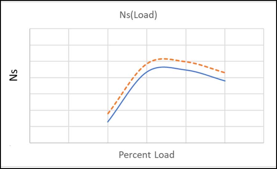 Figure 4
When the non-dimensional lift term, ΔP/P is calculated along the surge curve, many points can be found where no surge occurs as well as many where surge occurs at the same load, ΔP/P, and inlet guide vane position. So, if lift is non-dimensionalized, the control system has the potential to lose portions of the operating curve that could have been used to operate the chiller more efficiently. More importantly, this blocks out points needed to control the chiller at a given load and lift condition. The result is reduced turndown performance.
This demonstrates the principles of predictive optimization at the machine level as well as a second area of risk when using AI to optimize plants. Namely, using too little input can result in poorer efficiencies and poorer machine operation. The machine can "learn" the wrong thing without knowing it. If engineers optimize the plant predictively and use AI to validate the expected performance and identify deviations, they then have a cost-effective model to allow operators to achieve and maintain superior plant performance.
Results
In 2013, HGA installed the first plant using its predictive optimization approach. The University of Virginia North Grounds Plant demonstrated effective use of heat recovery chillers and a predictively optimized plant that reduced the annual average chiller plant all-in energy efficiency to less than 0.5 kW/ton. In 2015, UVA reported the measured energy use of the plant decreased by 48% due to the effective use of heat recovery chillers and the predictive optimization approach.
At the University of Wisconsin, HGA is implementing strategies based on the same principles that guide operators in the manual operation of four plants totaling 78,000 ton of capacity. Here, the cost savings potential is well over $1 million annually in energy cost savings.
Since 2013, HGA has implemented its predictive optimization approach on nearly every chiller plant the firm designs. It is a matter of designing plants well using a robust approach that can be implemented with any DDC system while not trying to over-control the plant. When applied with PLCs, engineers can take advantage of fault diagnostics to aid the operators in maintaining plant efficiencies. Savings are a function of the equipment, starting operating conditions, and modifications made (or not made) to the plant, ranging from 15%-30%, with simple paybacks generally under two years.


")