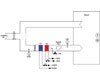
FIGURE 1. Schematic design of a typical constant volume AHU.
In which a mysterious five-degree difference is a $4,400/yr anomaly.
In last month’s column, I introduced the importance of trend-logging system operation over a multi-day period in order to observe subtleties not typically identified during onsite functional performance testing. I shared an example trend log for an air-handling system whose problems were obvious once they were graphed.
This month, I have another example which is a bit more understated. In order to fully appreciate what the trend graph tells us, it is important to understand the system and how it is intended to function. This particular AHU was a 5,000 cfm constant volume, single-zone air handler serving a very sensitive space requiring steady temperature and rh control. It was designed to operate with a constant minimum outside airflow, i.e., no economizer free cooling mode. Figure 1 is the schematic diagram of this system.
This system necessarily had heating, cooling, humidification, and dehumidification modes of operation, depending on space and outdoor conditions. There were very low thermal loads in the space (below grade, minimal occupancy, lights off unless occupied, etc.), therefore, much of the load was related to the minimal amount of outside air ventilation introduced for air quality and space pressurization purposes.
Figure 2 is the trend graph from this AHU over the course of approximately 10 days.
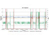
FIGURE 2. Trend graphic of a constant volume AHU.
With the AHU discharge temperature (purple) varying between 68°F and 72°, the space temperature (light blue) was very steady at its 70° setpoint. As such, it would be easy to conclude that this system was performing very well. The part that didn’t seem to fit was the mixed air temperature (orange), which was consistently about 5° lower than the discharge air temperature.
How is it that the mixed air temperature was being warmed that much with the chilled water valve 35% to 40% open? In such a small system, heat gain across the fan would not result in that type of heat load. This trend analysis allowed us to identify that the hot water control valve was leaking past. Even though its control system signal (the red line on the trend graph) was 0% open, the valve was physically not closing fully. If this had gone unnoticed by the commissioning process, the unnecessary hot water consumption and compensating chilled water consumption would have resulted in approximately $4,400/yr in wasted energy for the building owner.
In the best of all worlds, these types of trend logs would be collected and analyzed up to three times during the first year of operation, depending on the local climate: 1) during the winter; 2) during the summer; or 3) during a transition period, either spring or fall. Of course, the value of such analysis can also be carried into normal operations, and that is what I will address in next month’s column.ES